Introduction to simulation for experimental design using R
Etienne Low-Décarie
12 July 2018
Getting to know each other
Workshop
- Peer teaching and coding
- I am one of your peers… correct me when I am wrong! etc.
- Post its
- Challenges
- Don't look at solutions when given… -All material on github.com/low-decarie
Schedule
- Introduction
- Review of what makes a good study/experiment
- Experimentaly accounting for variability
- Some classical experimental designs
- ~10:30AM - 30 minute coffee break
- Justification of simulation for experimental design
- Basic experiment simulation using a spreadsheet
- Sampling in R
- Sampling a population
- Sampling from a distribution
- Repeated sampling and summary
- ~12:30PM - 60 minute lunch break
- Experimental design setup in R
- Simulating an experiment
- Scaling of predictors
- Replicated simulation
- Sensivitivy analysis
- ~15:30AM - 30 minute break
- Dojo and/or work on your experiment
To consult the statistician after an experiment is finished is often merely to ask him to conduct a post mortem examination. He can perhaps say what the experiment died of.
Sir Ronald Fisher, Presidential Address to the First Indian Statistical Congress, 1938. Sankhya 4, 14-17.

A good study/experiment
Good question / good hypothesis
- Falsifiable (testable)
- Common issue: absence of evidence is not evidence of absence
- Specific
- Powerful: generalizable, leading to prediction
- Empirical: direct to observation
- Plausible
Recognizing that not all studies are aimed at hypothesis testing.
- Falsifiable (testable)

A good study/experiment
- Avoids
- confounding variables
- experimental artifacts
- negative and positive controls
Issues with experimental design: gene expression studies in human populations
quantitative phenotype differs significantly between European-derived and Asian-derived populations
Common genetic variants account for differences in gene expression among ethnic groups
Issues with experimental design: gene expression studies in human populations
Interestingly, the arrays used to measure expression for the CEU [European-derived] individuals were primarily processed from 2003 to 2004,whereas the arrays used to measure expression for the ASN [Asian-derived] individuals were all processed in 2005–2006.
.
microarray batch effects appear to be completely confounded with population effects.”
On the design and analysis of gene expression studies in human populations
Issues with experimental design: sediment and herbivory

Sediment suppresses herbivory across a coral reef depth gradient
stratified with split plot treatment: air gun and air lift (vacuuming) control: plastic sheet protection

A good study/experiment
Accounts for variability
- replication
- randomization
- blocking
- stratification
- clustering
Issues with experimental design: experimental lakes
A good study/experiment
- Orthogonal explanatory variables (and interactions)
- Balance
- Sufficient power
- Replication vs pseudoreplication

Issues with experimental design: mesocosms
A good study/experiment
- Feasible!
- Results can be analyzed!
Issues with experimental design: my own experiments (1 of many issues)

Challenge with:
- analyzing species vs major taxonomic group
- repeated assays through time/generations
- multiple responses of interest
The effect of elevated CO2 on growth and competition in experimental phytoplankton communities
Classes (broad categories)
| Dependant\Independant | Continuous | Categorical |
|---|---|---|
| Continuous | Regression | ANOVA |
| Categorical | Logistic regression | Tabular |
A bestiary of classical experimental designs
Many are optimal experimental designs if all required experimental units are available
- repeated measures
- complete randomized design (CRD)
- complete (block)
- randomized:lattice, randomized complete block design (RCBD)
- blocking two variables: Latin Square, Youden, Graeco, BIB, , Cyclic, augmented block
- two variables of interest: split and strip plot Designs -incomplete:lattice, Alpha design

A bestiary of classical experimental designs
Famous failures of experimental design
Park grass experiment: -started by Lawes and Gilbert in 1856 at Rothemsted -162 years old
- pre-dates Fisher's work on experimental design at Rothemsted
- its original purpose was to investigate ways of improving the yield of hay by the application of inorganic fertilizers and organic manure.
Issues with experimental design: park grass
Challenge: Park grass
Park grass :
- What questions can you ask with the park grass experiment as it was designed?
Redesign park grass experiment:
- Given the experimental units provided (22 rows x 4 columns + 11 cells= 99) which of the park grass experiment questions (effect of N, P, Na, etc.) would you address and how?
- Given the questions park grass experiment, come up with a minimal design that addresses the historic set of questions/hypothesis
- Maybe start by listing the treatments and or associated questions. This could be done by specifying the complete model in R style formula syntax.
** WHat other famous failures of experimental design do you know? **
Coffee break
30 minutes

Park grass
Analysis despite flaws in experimental design:
Determinants of Species Richness in the Park Grass Experiment
Park grass inspired experiment using proper experimental design:
Effects of grassland management on plant C:N:P stoichiometry:implications for soil element cycling and storage (example publication, dozens of related publications)
Why simulate?
Why simulate?
- Eliminate the need for dice when playing Dungeons and Dragons
- Dry run of experimental design
- Good allocation of experimental effort
- vs optimal (ie algorithmic) allocation of experimental effort?
- vs power analysis (see vignette of
pwr
- Test/understand a statistical approach
- Explore theory/hypotheses
- Bad reason: Fake data…
Basic experiment simulation using a spreadsheet
- Effect of nitrogen and phosphorus on phytoplankton density in mesocosms
Challenge
Create a spreadsheet simulation of an experiment testing :
- testing the effect of nitrogen, phosphorus and [CO2] on chlorophyll in mesocosms
and/or
- testing difference between species in how (supra-optimal or full range) temperature affects their running spead
and/or
- the effect of gear choice and location on fisherman's catch
Issues with experiment simulation using a spreadsheet
What were issues you identified?
Issues with experiment simulation using a spreadsheet
- limited types of distributions
- tedious setup
- design (repetitive copy pasting)
- multiple trials (very long sheet)
- etc.
- challenge of scaling
- requires switching to R for downstream steps
- …
Sampling from a defined population in R
Throwing a six face die
Create the die
die <-seq(from=1, to=6, by=1)
Throw the die
sample(x=die, size=1, replace=T)
[1] 4
Sampling from a population
Throw the 1000 times and keep the results
die_results <- sample(x=die,
                      size=1000,
                      replace=T)
Sampling from a population
Plot the results
hist(die_results,
     breaks=seq(from=0.5,
                to=6.5,
                by=1))
3D die (just because we can)
#load TeachingDemos
require(TeachingDemos)
#create the die
rgl.die()
#roll the regular die
roll.rgl.die(steps=10)
TeachingDemos also contains a dice that throws ndice, rolls times
dice(rolls=3,
     ndice=4,
     sides=6,
     plot.it=T,
     load=rep(1, 6))
Challenges
- Throw a 10 faced die
- Throw a coin
- Throw cheaters die that produces 6 50% of the time
Solutions
die10 <-seq(from=1, to=10, by=1)
coin <- c("head", "tails")
p_dice<-c(1,1,1,1,1,5)
die_results <- sample(x=die,
                      size=1000,
                      replace=T,
                      prob= p_dice)
Sampling from a distribution
Normal distribution
rnorm(n = number of observations,
      mean = vector of means,
      sd = vector of means)
Sampling from a distribution
Normal distribution
sample_norm <- rnorm(n = 10000,
                     mean = 10,
                     sd = 1)
hist(sample_norm)
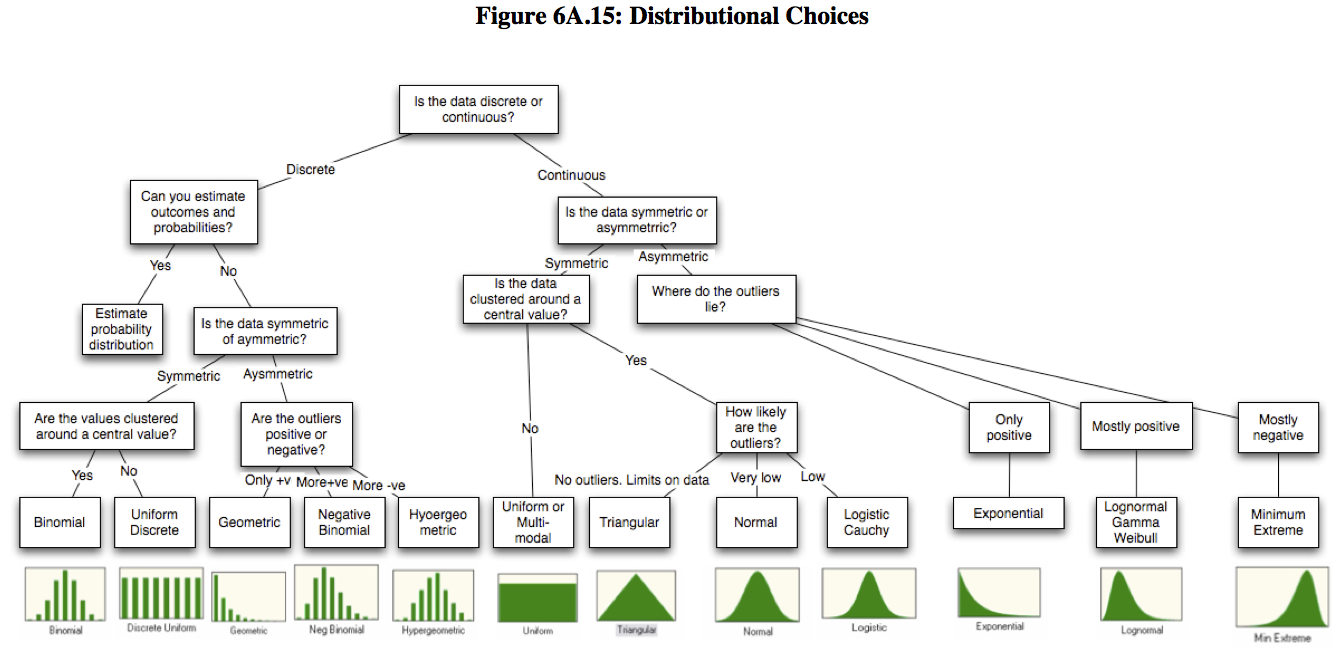
Bestiary of distributions
Available in base r:
beta beta, binomial binom, Cauchy cauchy, chi-squared chisq, exponential exp, Fisher F f, gamma gamma, geometric geom, hypergeometric hyper, logistic logis, lognormal lnorm, negative binomial nbinom, normal norm, Poisson pois, Student t t, uniform unif, Weibull weibull
Challenges
- Create a sample representing the number of dolphins seen per 10 hours of observation, for 100 observations (hint: assuming this is a number of independent events occurring in a fixed time)
- Create a sample representing the frequency of species in a quadrat (hint: assuming a few species will be very common and many species will be very rare)
Additional challenges:
- Plot these distributions.
- Repeat your sampling while the distribution while varying key parameters
- Plot summary statistics of your sampling with with various parameters
Solutions
1.
dolphins <- rpois(n = 1000,
                  lambda = 3)
hist(dolphins)
Solutions
2.
species <- rlnorm(n = 1000,
                  mean = 25,
                  sd=1)
hist(species)
Challenge
- Import one of your spreadsheet simulation into R
- Create a plot in R of the data simulated in Excel
- In
R, create a new column containing simulated values using a more sensible distribution of error
Lunch break
60 minutes
Simulating an experiment
design setup “manually”
Example 2 factors, 2 levels, 3 replicates, full factorial
one_replicate <- data.frame(factorA=factor(rep(c("FacA_Level1",
                                     "FacA_Level2"),
                                     3)),
                            factorB=factor(rep(c("FacB_Level1",
                                     "FacB_Level2", "FacB_Level3"),
                                     each=2)))
head(one_replicate)
      factorA     factorB
1 FacA_Level1 FacB_Level1
2 FacA_Level2 FacB_Level1
3 FacA_Level1 FacB_Level2
4 FacA_Level2 FacB_Level2
5 FacA_Level1 FacB_Level3
6 FacA_Level2 FacB_Level3
Alternatives:
- if conducting full factorial, use
expand.grid() - create design in spreadsheet and import
Need for scaling of predictors
require(cowplot)
one_replicate$response <- with(one_replicate,
                        as.numeric(factorA)*
                          as.numeric(factorB))
How to scale predictors
function to create scaled numeric predictors from all factors
num_scale_fact <- function(data_frame){
  ind <- sapply(data_frame, is.factor)
  data_frame[paste0("num_",names(data_frame[ind]))] <-
    lapply(data_frame[ind],
                                                              function(x)scale(as.numeric(x)))
  return(data_frame)
}
Results of scaling predictors
one_replicate <- num_scale_fact(one_replicate)

one_replicate$response <- with(one_replicate,
                        num_factorA*
                          num_factorB)
Adding error and replication
experiment1 <- NULL
for(i in LETTERS[1:3]){
  one_replicate$replicate <- factor(i)
  one_replicate$response <- with(one_replicate,
                        num_factorA*
                          num_factorB+rnorm(n = nrow(one_replicate), sd=2))
  experiment1 <- rbind(experiment1,one_replicate)
}
Avoid for loops in this context using the apltly named
replicate
Challenge
- Plot experiment 1
- Analyze experiment 1
- You know that factorA and factorB have an an interactive effect, can you detect this from this experiment?
- If you can detect an effect, what could you do to save money/time etc in this experiment?
- If you can not detect an effect, what would you need to do to detect the known effect?
Solution
1.
require(ggplot2)
p <- qplot(data=experiment1,
           x=factorA,
           y=response,
           colour=factorB,
           geom="boxplot")
print(p)
Solution
2.
fit <- aov(data = experiment1,
           response~factorA*factorB)
summary(fit)
                Df Sum Sq Mean Sq F value   Pr(>F)
factorA          1  0.000    0.00    0.00        1
factorB          2  0.000    0.00    0.00        1
factorA:factorB  2 12.500    6.25   24.98 5.28e-05 ***
Residuals       12  3.002    0.25
---
Signif. codes:  0 '***' 0.001 '**' 0.01 '*' 0.05 '.' 0.1 ' ' 1
Accelerate the process
Experimental setup using tools
require(AlgDesign)
experiment2 <- gen.factorial(levels=c(3,2,2),
                             nVars=3,
                             varNames=c("A","B","C"),
                             factors="all")
Replicate the whole experiments (trials)
create an expanded simulated data set and analyse each trial
create the experimental design
experiment_design <- gen.factorial(levels=c(3,2,2),
                            nVars=3,
                            varNames=c("A","B","C"),
                            factors="all")

experiment_design <- num_scale_fact(experiment_design)
Replicate the whole experiments design
- add replication and trial (replication of the experiment)
trial_rep <- expand.grid(trial=as.factor(1:1000),
                         rep=as.factor(1:5))

expand.grid.df <- function(...) Reduce(function(...) merge(..., by=NULL), list(...))

rep_exp1 <- expand.grid.df(trial_rep,experiment_design)
https://stackoverflow.com/questions/11693599/alternative-to-expand-grid-for-data-frames
Add a response
rep_exp1$response <- with(rep_exp1, num_A+num_B+num_B*num_C+num_A*num_B*num_C+rnorm(nrow(rep_exp1), sd=2))
Plotting the replicated experiment
p <- qplot(data=rep_exp1,
           x=A,
           y=response,
           colour = B,
           alpha=I(0.02),
           geom="jitter")+
  geom_line(aes(group=paste(trial, rep, B)),
             alpha=0.02)+
  facet_grid(. ~ C, labeller = label_both)
print(p)
Analysing the trials
require(broom)
require(dplyr)
fit_results <- rep_exp1 %>%
  group_by(trial) %>%
  do(tidy(aov(response~A*B*C, data=.)))

require(ggplot2)
p <- qplot(data = fit_results,
           x = p.value,
           binwidth=0.05)+
  facet_wrap(~term)
Analysing the trials
require(sjstats)
fit_results <- rep_exp1 %>%
  group_by(trial) %>%
  do(omega_sq(aov(response~A*B*C, data=.)))
Alternative methods to replicate the whole experiments
fit model to single experiment and use
simulatesimulate.lm : normal distribution with same MSE as original model
creat a base experiment
exp_d_rep <- do.call("rbind", replicate(3, experiment_design, simplify = FALSE))
exp_resp <- exp_d_rep
exp_resp$response <- with(exp_resp,
                       num_A+num_B+num_B*num_C+num_A*num_B*num_C+rnorm(nrow(exp_resp), sd=2))
Replicate with `simulate`
fit <- lm(response~A*B*C, data=exp_resp)
exp_sim <- cbind(exp_d_rep,simulate(fit,nsim = 10))

require(tidyr)
exp_sim <- gather(exp_sim,contains("sim_"), key = trial ,value = response)
Experimenting with experimental design
Sensitivity analysis of design: simulate a series of experimental design scenarios and see how it affects inference from the study.
Setup trials that vary in design
Lets get super meta: setup an experimental design for your sensitivity analysis experiment of your experiment
sens_setup <- expand.grid(trial=as.factor(1:100),
                         replication=c(3:10),
                         error=c(0.1,0.5,1,5,10))
Calcualte the response for different design values
Setup a function
f_rep_error <- function(rep,error){
  rep_exp <- expand.grid.df(data.frame(rep=rep, replicate=1:rep),experiment_design)
  rep_exp$response <- with(rep_exp, num_A+num_B+num_B*num_C+num_A*num_B*num_C+rnorm(nrow(rep_exp), sd=error))
  return(rep_exp)
}
Apply the function to individual trials
trial_rep_error <- sens_setup %>% group_by(trial, replication, error) %>%
  do(with(.,f_rep_error(replication, error)))
Sensitivity analysis of experimental design
or experimenting with experimental design
require(broom)
require(dplyr)
fit_results <- trial_rep_error %>%
  group_by(trial, rep, error) %>%
  do(tidy(aov(response~A*B*C, data=.)))
Accelerate the process in specific cases
Optimize the design using tools
For certain types of design, the allocation of experimental units can be optimized using established algorithsm.
For example,in some cases, a full factorial design can be reduced to a carefully selected subset of cases with only a marginal effect on estimated parameters.
see R vignette("AlgDesign")
- optBlock {AlgDesign}
- optFederov {AlgDesign}
Challenges
- instead of
gen.factorialuse one of the optimize incomplete factorial designs using the same setuprep_exp1- can you detect the all the same effects?
- are the parameter estimates similar?
- does the use of non-normaly distributed error (eg. poisson) affect your interpreation using
aov? - any difference with numeric rather than factor predictors?
- what are the effect of a non-linear interaction with one of your predictors?
- what are the effect of heteroscedasticity (eg. correlation of variance with one of the predictors)?
Coffee break
30 minutes

Dojo
Dojo: deliberate practice
- pair/team coding
Alternative: pair/team coding on each other's experiments (turns focusing on each experiment in the team).
Dojo 1
Produce an optimal design for the treatments in the Park Grass experiment
Dojo 2
Design an experiment to:
- Detect the effect of biodiversity on ecosystem process
- Include a species that has a high contribution to ecosystem function compared to the average of all other species
- Include a pair of species that seperatly do not contribute to the process, but together have a strong impact on diversity
- How many levels of biodiversity should your experiment contain?
- How many replicate communities are needed at each level?
- Can blocking help distinguish between composition effects (eg. sampling effect) and diversity effect?
Dojo 3
Redesign the experiment from your favourite recent publication
- Use the same number of experimental units and try to improve on the design
- Were the authors lucky? Insert problems into the study (eg. other distribution, loss of a replicate). Do you consistently get the same results.